Polynomial Regression, Overfitting, and Regularization#
Polynomial Regression#
Slides: Polynomial Regression, Overfitting and Regularization 1
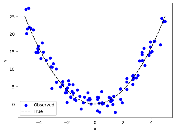
ข้อมูลจำนวนมากที่พบเจอในการทำงานจริง มักมีความสัมพันธ์ที่ซับซ้อน ซึ่งเมื่อนำมา plot ดูแล้วอาจจะมีหน้าตาที่ไม่สอดคล้องกับโมเดลเชิงเส้น ดังตัวอย่างด้านล่าง ที่ \(y\) ถูกสร้างมาจากสมการ \(y=x^2\)
import sys
import numpy as np
from numpy.linalg import norm
import matplotlib.pyplot as plt
from sklearn.linear_model import LinearRegression
from sklearn.preprocessing import PolynomialFeatures

import ipywidgets as widgets  # ใช้สำหรับการทำ interactive display

np.random.seed(777) # ตั้งค่า random seed เอาไว้ เพื่อให้การรันโค้ดนี้ได้ผลเหมือนเดิม
def generate_sample_poly(x, w_list, include_noise=True, noise_level=2):

    # จำลองการใส่สัญญาณรบกวนเข้าไป
    if include_noise:
      noise = noise_level*np.random.randn(*x.shape)
    else:
      noise = 0

    y = 0

    # ค่อย ๆ เติม พจน์ที่มีเลขยกกำลังต่าง ๆ กัน ตาที่กำหนดไว้ใน w_list
    for curr_order, curr_w in enumerate(w_list):
      y += curr_w* (x**curr_order)

    return y + noise


num_samples = 100
w = [0, 0, 1]
x = 10*np.random.rand(num_samples,1) - 5
y = generate_sample_poly(x, w, include_noise=True)

# สร้างข้อมูลที่ไม่มีสัญญาณรบกวนมาเปรียบเทียบ
y_true = generate_sample_poly(x, w, include_noise=False)

# สร้างข้อมูลที่ไม่มีสัญญาณรบกวนมาแบบละเอียด เพื่อใช้ในการวาดกราฟ (เส้นประสีดำ)
x_whole_line = np.linspace(-5, 5, 100)
y_true_whole_line = generate_sample_poly(x_whole_line, w, include_noise=False)

# Plot ข้อมูล x, y ที่มีอยู่
fig, ax = plt.subplots()
ax.scatter(x, y, c='b', label='Observed')
ax.plot(x_whole_line, y_true_whole_line, 'k--', label='True' )
ax.set(xlabel='x', ylabel='y')
ax.legend()
plt.show()
หากเรานำเอาสมการเส้นตรง \( y = \hat{w_0} + \hat{w_1} x\) มาอธิบายข้อมูลประเภทนี้ จะส่งผลให้เกิดความคาดเคลื่อนได้
model_linear = LinearRegression()

# ให้โมเดลหาค่า w_0 and w_1 จากข้อมูล (x,y) ทั้งหมดที่มี
model_linear.fit(x, y)

w0_hat = model_linear.intercept_[0]
w1_hat = model_linear.coef_[0][0]

print(f"Estimated slope {w1_hat:0.2f}\n")
print(f"Estimated intercept {w0_hat:0.2f}")

# ใช้โมเดลทำนายค่า y จากค่า x วิธีที่ 2
y_hat = model_linear.predict(x)

# ฟังก์ชันสำหรับวัด mean squared error ระหว่างค่าที่ทำนายได้ (y_hat) และค่าผลเฉลย y
def mse(y, y_hat):
  return np.mean((y-y_hat)**2)/y.shape[0]

mse_val = mse(y_true, y_hat)

# แสดงผลการทำนาย
fig, ax = plt.subplots()
ax.scatter(x, y, c='b', label='Observed')
ax.set(xlabel='x', ylabel='y')
ax.scatter(x, y_hat, c='r', label='Predicted')
ax.plot(x_whole_line, y_true_whole_line, 'k--', label='True' )
ax.legend()
ax.set_title(f"The error as measured by MSE = {mse_val:0.4f} w.r.t the true relationship")
plt.show()
Estimated slope -0.18

Estimated intercept 8.10
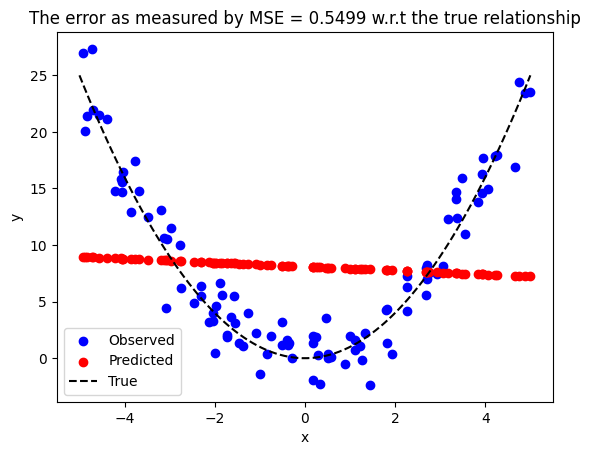
จะพบว่าโมเดลเส้นตรงนั้นไม่สอดคล้องกับข้อมูลที่เรามีอยู่ สังเกตได้จาก
ข้อมูลสีแดงที่โมเดลทำนายมา ไม่สอดคล้องกับข้อมูลจุดสีน้ำเงิน
ค่า mean squared error (MSE) สูง
จึงมีความจำเป็นที่จะต้องหาวิธีที่จะอธิบายความสัมพันธ์แบบที่ไม่เป็นเส้นตรง (nonlinear relationship) ได้
ในส่วนนี้เราจะลองใช้โมเดลที่มีสมการดังนี้ \(y = \hat{w_0} + \hat{w_1}x+ \hat{w_2}x^2+ ...+ \hat{w_p} x^p\)
ถ้า \(p = 1\) เราจะได้โมเดล \(y = \hat{w_0} + \hat{w_1} x\) ในการพัฒนาโมเดลในกรณีนี้ เราจะต้องหาค่า \(\hat{w_0}\) (จุดตัดแกน \(y\) ที่เหมาะสม) และค่า \(\hat{w_1}\) (ค่าความชันของเส้นตรง) ได้เหมือนกับตัวอย่างที่ผ่าน ๆ มา
ถ้า \(p = 2\) เราจะได้โมเดล \(y = \hat{w_0} + \hat{w_1} x + \hat{w_2} x^2\) ในกรณีนี้เราจะต้องหาค่า \(\hat{w_0}, \hat{w_1}\) และ \(\hat{w_2}\)
ถ้า \(p = 3\) เราจะได้โมเดล \(y = \hat{w_0} + \hat{w_1} x + \hat{w_2} x^2 + \hat{w_3} x^3\) ในกรณีนี้เราจะต้องหาค่า \(\hat{w_0}, \hat{w_1}, \hat{w_2}\) และ \(\hat{w_3}\)
สังเกตได้ว่ายิ่ง \(p\) มีค่าสูงมากขึ้น จำนวนตัวแปรที่เราต้องหาค่าเพื่อพัฒนาโมเดลจะเพิ่มขึ้น
หากเราสนใจประมาณค่า \(\hat{w}\) โมเดลนี้จะถือว่าเป็นโมเดลเชิงเส้น (ในโมเดลไม่มีพจน์ประเภทที่เลขชี้กำลังของ \(\hat{w}\) มีค่าไม่ใช่ \(0\) หรือ \(1\) เลย เช่น ไม่มี \(\hat{w^2}, \hat{w^3}, ..., \hat{w^p}\) เลย) ทำให้เราสามารถใช้ LinearRegression ในการแก้ปัญหาได้เหมือนเดิม เพียงแต่เราต้องมีการปรับแก้ input ก่อน
ข้อมูลทางเทคนิคเพิ่มเติม
ใน part ที่แล้วเราได้เห็นแล้วว่า multiple linear regression มีสมการเป็น
หากกำหนดให้ \(z_i = x^i\) จะส่งผลให้เราสามารถเขียนโมเดลใหม่ได้เป็น
เราเห็นว่าทั้งสองสมการหน้าตาคล้ายกันมาก และเรารู้วิธีใช้ LinearRegression มาหาค่า \(\hat{w_0}, \hat{w_1}, ..., \hat{w_p}\) ของสมการแรกได้ เราก็ควรจะใช้ LinearRegression มาหาค่า \(\hat{w_0}, \hat{w_1}, ..., \hat{w_p}\) ของสมการที่ 2 ได้เช่นกัน
ในส่วนถัดไป เราจะลองนำเอาโมเดล \(y = \hat{w_0} + \hat{w_1} z_1+ \hat{w_2} z_2 + \hat{w_3} z_3 + \hat{w_4} z_4\) มาใช้กับข้อมูลจากข้อก่อนหน้า
# ฟังก์ชันสำหรับ fit โมเดล polynomial ที่มี order ที่กำหนด และ ทำนายผลของโมเดลหลังจากถูกสอนด้วย training data แล้ว
def fit_and_predict_polynomial(x_train, # ค่า x ที่ใช้เป็น input ของโมเดล (จาก training data)
                               y_train, # ค่า y ที่ใช้เป็นเฉลยให้โมเดล (จาก training data)
                               poly_order=4, # ค่า order ของ polynomial ที่เราใช้
                               x_test_dict=None, # Python dictionary ที่ใช้เก็บชุดข้อมูลที่เราอยากจะนำมาทดสอบ โดยสามารถเลือกชุดข้อมูลผ่าน key ของ dictionary นี้
                               y_test_dict=None): # Python dictionary ที่ใช้เก็บชุดข้อมูลที่ค่า y ที่เป็นเฉลยของข้อมูลที่นำมาทดสอบ โดยสามารถเลือกชุดข้อมูลผ่าน key ของ dictionary นี้

    # สร้างตัวแปรประเภท Python dictionary สำหรับเก็บค่า output ของฟังก์ชันนี้
    mse_dict = {} # ค่า mse
    out_x = {} # ค่า x ที่ใช้เป็น input ของโมเดล
    out_y_hat = {} # ค่า y ที่โมเดลตอบมา
    out_y = {} # ค่า y ที่เป็นเฉลย

    # สร้างโมเดลสำหรับแปลงจาก x เป็น z
    extract_poly_feat = PolynomialFeatures(degree=poly_order, include_bias=True)

    # แปลงจากค่า x ให้กลายเป็น z
    z_train = extract_poly_feat.fit_transform(x_train)

    # สร้างโมเดล y = w_0 + w_1*z_1 + w_2 * z_2 + ...
    model_poly = LinearRegression()

    # สอนโมเดลจาก training data ที่ input ถูก transfrom จาก x มาเป็น z แล้ว
    model_poly.fit(z_train, y_train)

    # ทดสอบโมเดลบน training data
    y_hat_train = model_poly.predict(z_train)

    # ถ้าเกิดว่า user ไม่ได้ให้ test data มา จะใช้ training data เป็น test data
    if x_test_dict is None:
        x_test_dict = {}
        y_test_dict = {}

    # เพิ่ม training data เข้าไปใน test_dict เพื่อที่จะใช้เป็นหนึ่งในข้อมูลสำหรับที่จะให้โมเดลลองทำนาย
    x_test_dict['train'] = x_train
    y_test_dict['train'] = y_train

    # ทดสอบโมเดลบนข้อมูลแต่ละชุดข้อมูล (แต่ละชุดข้อมูลถูกเลือกจาก key ของ dictionary)
    for curr_mode in x_test_dict.keys():

        # แปลงค่า x ให้เป็น z เหมือนขั้นตอนด้านบนที่เรา fit โมเดล
        z_test = extract_poly_feat.fit_transform(x_test_dict[curr_mode])

        # ทำนายค่า y โดยใช้โมเดล
        y_hat_test = model_poly.predict(z_test)

        # คำนวณค่า mse บน test data
        mse_dict[curr_mode] = mse(y_test_dict[curr_mode], y_hat_test)

        # เตรียมข้อมูลเป็น output ของฟังก์ชันนี้ เผื่อเรียกใช้ภายหลัง เช่น การนำเอาข้อมูลไป plot
        out_x[curr_mode] = x_test_dict[curr_mode] # เก็บค่า x ที่นำมาทดสอบ
        out_y_hat[curr_mode] = y_hat_test # เก็บค่า y ที่โมเดลทำนายออกมา
        out_y[curr_mode] = y_test_dict[curr_mode] # เก็บค่า y ที่เป็นผลเฉลย

    return out_x, out_y_hat, out_y, mse_dict, model_poly.coef_[0]


# polynomial order
poly_order = 4
out_x, out_y_hat, out_y, mse_dict, model_coeffs = fit_and_predict_polynomial(x,
                                                                             y,
                                                                             poly_order)

# แสดงผลการทำนาย
fig, ax = plt.subplots()
ax.scatter(out_x['train'], out_y_hat['train'], c='r', label='Predicted (poly)')
ax.scatter(x, y, c='b', label='Observed')
ax.plot(x_whole_line, y_true_whole_line, 'k--', label='True' )
ax.set(xlabel='x', ylabel='y')
ax.legend()
ax.set_title(f"The error as measured by MSE = {mse_val:0.4f}")
plt.show()

# แสดงค่า w ของโมเดล
print(f"[w_0, w_1, ...]= {model_coeffs}")
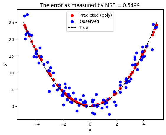
[w_0, w_1, ...]= [ 0. -0.00433819 1.03139417 -0.00184097 -0.00225545]
ถึงแม้ว่าเราจะใช้โมเดลที่มีสมการเป็น \(\hat{y} = \hat{w_0} + \hat{w_1}x + \hat{w_2} x^2 + \hat{w_3} x^3 + \hat{w_4}x^4\) เราพบว่าโมเดลประมาณค่าของ \(\hat{w_3}\) และ \(\hat{w_4}\) เป็นตัวเลขที่มีค่าใกล้ศูนย์มาก ๆ ซึ่งแปลว่าโมเดลเราจะมีพฤติกรรมคล้ายคลึงกับโมเดลที่มีสมการเป็น \(\hat{y} = \hat{w_0} + \hat{w_1}x + \hat{w_2} x^2\)
หมายเหตุ เราจะเรียกข้อมูลที่ใช้สำหรับสอนโมเดลว่า training data \((x_{train},y_{train})\) และจะเรียกข้อมูลที่ใช้สำหรับทดสอบโมเดลว่า test data \((x_{test},y_{test})\)
Overfitting#
หากสังเกตดู code ด้านบนจะพบว่าข้อมูลที่เราใช้สำหรับสอนโมเดลนั้นมีจำนวนค่อนข้างมาก เมื่อเทียบกับจำนวนตัวแปร (มีข้อมูล 100 จุด แต่มีจำนวนตัวแปรแค่ 5 ตัว ซึ่งประกอบไปด้วย \(\hat{w_0}, \hat{w_1}, \hat{w_2}, \hat{w_3}\) และ \(\hat{w_4}\))
ในส่วนถัดไป เราจะลองใช้วิธีการเดิม โดยที่ข้อมูลนั้นจะยังถูกสร้างจากสมการ \(y=x^2\) เหมือนเดิม แต่มีจำนวนจุดข้อมูลที่น้อยลงมาก (จาก 100 จุด เหลือเป็น 10 จุด) และเราจะลองเปลี่ยนค่า polynomial order ไปเรื่อย ๆ
# มีจำนวนข้อมูลแค่ 10 จุด
num_samples = 10
w = [0, 0, 1]
x_train = 10*np.random.rand(num_samples,1) - 5
y_train = generate_sample_poly(x_train, w, include_noise=True)

# สร้างข้อมูลที่ไม่มีสัญญาณรบกวนมาเปรียบเทียบ
x_whole_line = np.linspace(-5,5,100)
y_true_whole_line = generate_sample_poly(x_whole_line, w, include_noise=False)

# ใส่แถบสำหรับปรับค่า w1_hat และ w2_hat รวมถึงช่องสำหรับให้เลือกว่าจะโขว์เส้นความสัมพันธ์ระหว่าง x และ y ที่แท้จริงหรือไม่
@widgets.interact(p=widgets.IntSlider(2, min=1, max=50),
                  show_true_line=widgets.Checkbox(True, description='Show true data'))
def plot_poly_results(p, show_true_line):

    # fit โมเดล และให้โมเดลทำนายค่า y ออกมา
    curr_outputs = fit_and_predict_polynomial(x_train, y_train, p)

    # ดึงเอา output ของฟังก์ชันออกมา
    out_x = curr_outputs[0] # ค่า x ที่ถูกใช้ทดสอบโมเดล
    out_y_hat = curr_outputs[1] # ค่า y ที่โมเดลทำนายออกมา
    mse_dict = curr_outputs[3] # ค่า mse ระหว่างสิ่งที่โมเดลทำนายออกมาและผลเฉลย

    # สร้าง figure
    fig, ax = plt.subplots(figsize=(4,4))

    # Plot ข้อมูลที่เราใช้ fit โมเดล (สอนโมเดล)
    ax.scatter(x_train, y_train, c='b', label='Observed')

    # Plot ข้อมูลที่โมเดลทำนายค่าออกมา
    ax.scatter(out_x['train'], out_y_hat['train'], c='r', label='Predicted (poly)')

    # Plot ข้อมูลที่ไม่มี noise สำหรับเป็น reference ไว้ดู
    if show_true_line:
        ax.plot(x_whole_line, y_true_whole_line, 'k--', label='True')

    ax.set(xlabel='x', ylabel='y')
    ax.set_title(f"Order = {p} with MSE = {mse_dict['train']:0.4f}")
    ax.legend()
    plt.show()
ทีนี้เราลองเอาผลจากค่า polynomial order ของโมเดลที่แตกต่างกันมาเปรียบเทียบกันดู
# ลองทดสอบเปลี่ยนค่า polynomial order
poly_order_list = [1, 2, 4, 8, 10, 15]
mse_list = [] # ตัวแปรสำหรับเก็บค่า mse

fig, ax = plt.subplots(2,3, figsize=(15, 12))
fig_row, fig_col = 0, 0

for idx, curr_poly_order in enumerate(poly_order_list):

    # fit โมเดล และให้โมเดลทำนายค่า y ออกมา
    curr_outputs = fit_and_predict_polynomial(x_train, y_train, curr_poly_order)

    # ดึงเอา output ของฟังก์ชันออกมา
    out_x = curr_outputs[0] # ค่า x ที่ถูกใช้ทดสอบโมเดล
    out_y_hat = curr_outputs[1] # ค่า y ที่โมเดลทำนายออกมา
    mse_dict = curr_outputs[3] # ค่า mse ระหว่างสิ่งที่โมเดลทำนายออกมาและผลเฉลย

    # เก็บค่า mse ของแต่ละชุดข้อมูลที่นำมาทดสอบที่มีค่า order ของ polynomial ที่แตกต่างกัน
    mse_list.append(mse_dict['train'])

    # แสดงผล
    if idx % 3 == 0 and idx != 0:
        fig_col = 0
        fig_row += 1

    # Plot ข้อมูลที่เราใช้ fit โมเดล (สอนโมเดล)
    ax[fig_row, fig_col].scatter(x_train, y_train, c='b', label='Observed')

    # Plot ข้อมูลที่โมเดลทำนายค่าออกมา
    ax[fig_row, fig_col].scatter(out_x['train'], out_y_hat['train'], c='r', label='Predicted (poly)')

    # Plot ข้อมูลที่ไม่มี noise สำหรับเป็น reference ไว้ดู
    ax[fig_row, fig_col].plot(x_whole_line, y_true_whole_line, 'k--', label='True')

    ax[fig_row, fig_col].set(xlabel='x', ylabel='y')
    ax[fig_row, fig_col].set_title(f"Order = {curr_poly_order} with MSE = {mse_dict['train']:0.4f}")

    ax[fig_row, fig_col].legend()

    fig_col += 1

# แสดงผล mse vs poly order
plt.figure()
plt.plot(poly_order_list, mse_list)
plt.xlabel('Polynomial order')
plt.ylabel('MSE')
plt.grid()
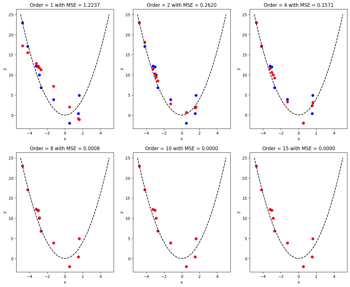
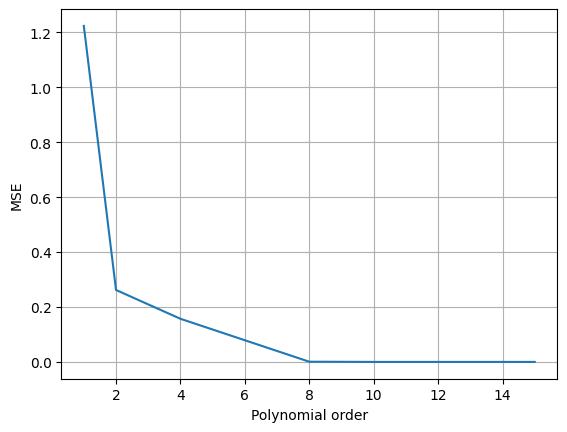
จากผลการทดสอบเปลี่ยนค่า polynomial order ของโมเดล จะพบว่าค่า MSE ที่ถูกทดสอบมีค่าน้อยลงเรื่อยๆ จนเหลือ \(0\) ที่ polynomial order \(= 15\)
แสดงว่าในการใช้งานจริงเราควรจะใช้ค่า order สูงๆ เนื่องจากมีค่า MSE น้อยที่สุดใช่หรือไม่
คำตอบคือไม่
MSE ที่เรานำมาใช้คำนวณเป็น MSE จาก training data ซึ่งเป็นข้อมูลที่โมเดลใช้ในการหาค่า \(\hat{w}\) ซึ่งการที่โมเดลมีค่า MSE ต่ำมากๆ แสดงว่าโมเดลมีความสามารถในการ fit ข้อมูลที่โมเดลเคยเห็นมาแล้วได้เป็นอย่างดี แต่ถ้าเกิดว่าเรานำเอาค่า \(x\) ตัวใหม่ที่โมเดลไม่เคยเห็นมาก่อน โมเดลที่มี order สูงจะยัง fit ได้ดีหรือไม่
เราจะลองเขียนโปรแกรมเพื่อทดสอบดู
# สร้างข้อมูลสำหรับใช้ทดสอบจำนวนมาก
x_test = np.reshape(np.linspace(-10,10,1000), (-1,1))
y_test = generate_sample_poly(x_test, w, include_noise=True)
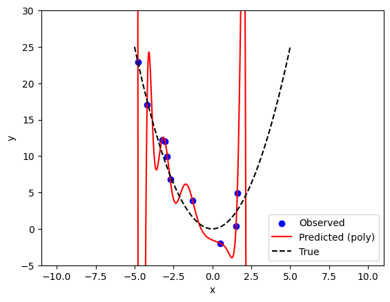
# จากการทดลองด้านบน เราพบว่า poly_order = 15 มีค่า MSE ที่ต่ำที่สุด
poly_order = 15
# fit โมเดล และให้โมเดลทำนายค่า y ออกมา
curr_outputs = fit_and_predict_polynomial(x_train, y_train, curr_poly_order, {'test': x_test}, {'test': y_test})
# ดึงเอา output ของฟังก์ชันออกมา
out_x = curr_outputs[0] # ค่า x ที่ถูกใช้ทดสอบโมเดล
out_y_hat = curr_outputs[1] # ค่า y ที่โมเดลทำนายออกมา
mse_dict = curr_outputs[3] # ค่า mse ระหว่างสิ่งที่โมเดลทำนายออกมาและผลเฉลย
model_coeffs = curr_outputs[4] # ค่า coefficients ของโมเดล
# แสดงผลการทำนาย
fig, ax = plt.subplots()
ax.scatter(x_train, y_train, c='b', label='Observed')
ax.plot(out_x['test'], out_y_hat['test'], c='r', label='Predicted (poly)')
ax.plot(x_whole_line, y_true_whole_line, 'k--', label='True')
ax.set(xlabel='x', ylabel='y')
ax.legend()
ax.set_ylim(-5, 30)
plt.show()
# แสดงค่า w ของโมเดล
print(f"[w_0, w_1, ...]= {model_coeffs}")
[w_0, w_1, ...]= [ 4.38918870e-07 -9.16803517e-01  5.25232344e-01 -9.06545642e-01
  5.91847282e-01 -7.01295262e-01  3.80429515e-02  1.41867825e-02
 -6.74743217e-01  3.47335771e-02  3.91400155e-01  1.12787498e-01
 -3.56448876e-02 -2.30436108e-02 -4.11080381e-03 -2.51657502e-04]
จากการทดสอบด้านบนจะพบว่าโมเดลมี training error เป็นศูนย์ (สังเกตได้จากการที่เส้นสีแดงวิ่งผ่านจุดสีน้ำเงินทั้งหมด) แต่จะเห็นได้ว่าเส้นสีแดงนั้น ไม่สอดคล้องกับ โมเดลจริง (เส้นประสีดำ) เลย
ปัญหาที่โมเดลสามารถให้คำตอบที่ถูกต้องบน training data แต่มีปัญหาในการใช้งานกับข้อมูลที่ไม่ได้ถูกนำมาสอนนั้น มีชื่อเรียกว่าปัญหา overfitting
นอกจากปัญหา overfitting แล้ว เราก็ยังมี underfitting ซึ่งเป็นปัญหาที่เราจะเจอในกรณีที่โมเดลอาจจะมีความซับซ้อนน้อยเกินไป จนไม่สามารถเรียนรู้ที่จะให้คำตอบที่ถูกต้องแม้กระทั่งกับ training data ซึ่งเป็นสิ่งที่ใช้สอนโมเดล
Code ส่วนถัดไปสร้างภาพสรุป concept นี้
# สร้างข้อมูลสำหรับใช้ทดสอบจำนวนมาก
x_test = np.reshape(np.linspace(-10, 10, 1000), (-1, 1))
y_test = generate_sample_poly(x_test, w, include_noise=True)

# Underfit
curr_outputs = fit_and_predict_polynomial(x_train, y_train, 1, {'test': x_test}, {'test': y_test})
x_test_underfit = curr_outputs[0]['test']
y_hat_test_underfit = curr_outputs[1]['test']

# Well fit
curr_outputs = fit_and_predict_polynomial(x_train, y_train, 2, {'test': x_test}, {'test': y_test})
x_test_wellfit = curr_outputs[0]['test']
y_hat_test_wellfit = curr_outputs[1]['test']

# Overfit
curr_outputs = fit_and_predict_polynomial(x_train, y_train, 15, {'test': x_test}, {'test': y_test})
x_test_overfit = curr_outputs[0]['test']
y_hat_test_overfit = curr_outputs[1]['test']

# แสดงผลการทำนาย
fig, ax = plt.subplots(1, 3, figsize=(18, 6))

ax[0].scatter(x_train, y_train, c='b', label='Observed')
ax[0].plot(x_test_underfit, y_hat_test_underfit, c='r', label='Predicted (poly)')
ax[0].plot(x_whole_line, y_true_whole_line,'k--', label='True')
ax[0].set(xlabel='x', ylabel='y')
ax[0].legend()
ax[0].set_ylim(-5, 30)
ax[0].set_title('Underfitting')

ax[1].scatter(x_train, y_train, c='b', label='Observed')
ax[1].plot(x_test_wellfit, y_hat_test_wellfit, c='r', label='Predicted (poly)')
ax[1].plot(x_whole_line, y_true_whole_line, 'k--', label='True')
ax[1].set(xlabel='x', ylabel='y')
ax[1].legend()
ax[1].set_ylim(-5, 30)

ax[2].scatter(x_train, y_train, c='b', label='Observed')
ax[2].plot(x_test_overfit, y_hat_test_overfit, c='r', label='Predicted (poly)')
ax[2].plot(x_whole_line, y_true_whole_line, 'k--', label='True')
ax[2].set(xlabel='x', ylabel='y')
ax[2].legend()
ax[2].set_ylim(-5, 30)
ax[2].set_title('Overfitting')

plt.show()
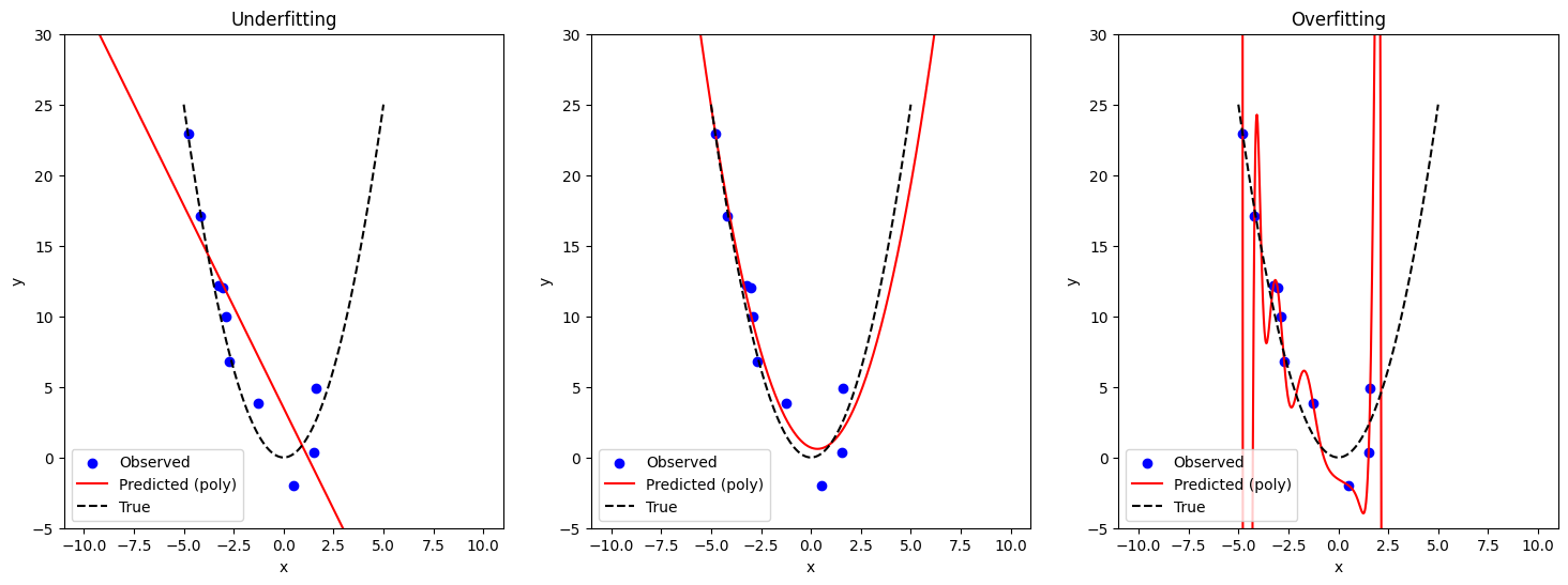
ในกรณีที่เราเจอปัญหา underfitting วิธีแก้ปัญหาวิธีหนึ่งที่ได้รับความนิยมมากก็คือ การเลือกใช้โมเดลที่ซับซ้อนมากยิ่งขึ้น เช่น การเพิ่มจำนวนตัวแปรในโมเดล หรือในตัวอย่างนี้ก็คือการเพิ่ม order ของ polynomial
ในกรณีที่เราเจอปัญญา overfitting เรามีวิธีบรรเทาปัญหานี้หลายวิธี เช่น
การลดจำนวนตัวแปรในโมเดล (สำหรับ polynomial ก็คือการลด order)
การใช้เทคนิค regularization
Regularization#
Slides: Polynomial Regression, Overfitting and Regularization 2
ที่ผ่านมา เราหาค่า \(\hat{w}\) ที่เหมาะสมในโมเดล polynomial regression โดยการหาค่าต่ำสุดของ loss function ที่วัดความแตกต่างระหว่างค่าที่โมเดลทำนายออกมา (\(\hat{y_i}\)) และค่าที่เรา observed มา (\(y_i\)) โดยการคำนวณ mean-squared error หรือ
ซึ่งเราใช้ PolynomialFeatures ร่วมกับ LinearRegression ของ scikit-learn ในการหาค่า \(\hat{w}\) เหล่านั้น
จากตัวอย่างที่เรากำหนดให้ \(p=15\) ซึ่งเป็น polynomial ที่มี order = 15 หรือมีตัวแปรทั้งหมด 16 ตัว (\(\hat{w_0}, \hat{w_1}, ..., \hat{w_{15}}\)) เราพบปัญหา overfitting
ในตัวอย่างนี้เราจะลองใช้เทคนิค regularization ทดลองดูว่าเราจะสามารถบรรเทาปัญหา overfitting ที่พบเจอได้หรือไม่
ในรูปแบบมาตรฐานของการใช้เทคนิค regularization เราจะเปลี่ยนหน้าตาของ loss function ไปจากเดิม โดยการเพิ่มพจน์ (term) เข้าไป เช่น การเปลี่ยน loss function ไปเป็น \(L(y, \hat{y}) =\frac{1}{n}\sum_{i=1}^{n}\left(y_{i}-(\hat{w_0} + \hat{w_1}x_i + \hat{w_2} x_i^2 + ... + \hat{w_{15}} x_i^{15})\right)^{2} +λ R(\mathbf{\hat{w}})\)
ในที่นี้เราใช้ \(\mathbf{\hat{w}}\) เพื่ออ้างอิงถึง \(\hat{w_0}, \hat{w_1}, ..., \hat{w_{15}}\) พร้อมกัน
เราเรียก \(R(\mathbf{\hat{w}})\) ว่าเป็น regularization term ซึ่ง regularization ที่เราจะเห็นได้บ่อยที่สุด ประกอบด้วย
\(R(\mathbf{\hat{w}})=\|\mathbf{\hat{w}}\|^2_2 = \hat{w_0}^2 + \hat{w_1}^2 + ... + \hat{w_{15}}^2\) ซึ่งมีชื่อเรียกว่า L2 regularization หรือ Tikhonov regularization
\(R(\mathbf{\hat{w}})=\|\mathbf{\hat{w}}\|_1 = |\hat{w_0}| + |\hat{w_1}| + ... + |\hat{w_{15}}|\) หรือ L1 regularization
ถ้าหากเราเพิ่ม L2 regularization term เข้าไป จะส่งผลให้โจทย์ที่เราต้องแก้เปลี่ยนหน้าตาไปเป็น
\(\min_{\mathbf{\hat{w}}}\frac{1}{n}\sum_{i=1}^{n}\left(y_{i}-(\hat{w_0} + \hat{w_1}x_i + \hat{w_2} x_i^2 + ... + \hat{w_{15}} x_i^{15})\right)^{2} +λ (\hat{w_0}^2 + \hat{w_1}^2 + ... + \hat{w_{15}}^2)\)
ซึ่งเราเรียกว่า Ridge regression
ในการหาค่าต่ำสุดของฟังก์ชันอันใหม่นี้ เราต้องการให้ทั้ง term ที่ 1 และ term ที่ 2 มีค่าที่ต่ำ
โดยที่มี \(λ \ge 0\) เป็นตัวเลขที่ใช้ balance ว่า เราจะให้ความสำคัญกับ term ที่ 1 หรือ term ที่ 2 มากกว่ากัน
ถ้าหากเราเพิ่ม L1 regularization term เข้าไป โจทย์ของเราจะเปลี่ยนไปเป็น
\(\min_{\mathbf{\hat{w}}}\frac{1}{n}\sum_{i=1}^{n}\left(y_{i}-(\hat{w_0} + \hat{w_1}x_i + \hat{w_2} x_i^2 + ... + \hat{w_{15}} x_i^{15})\right)^{2} +λ (\hat{|w_0|} + \hat{|w_1|} + ... + \hat{|w_{15}}|)\)
ซึ่งเราจะเรียกว่า Least Absolute Shrinkage and Selection Operator (LASSO) โดยเราสามารถใช้ \(λ\ge0\) เป็นตัวกำหนดความสำคัญของแต่ละ term ได้เช่นกัน
ตัวอย่าง สมมติเราใช้ L2 regularization โจทย์ของเราก็คือ
เรามาลองพิจารณาหลายๆ กรณีสุดโต่ง 2 กรณี
หากกำหนดให้ \(λ=0\) โจทย์ของเราจะกลายเป็น
เราจะได้ loss function ที่ไม่สนใจ regularization term หรือ term ที่ 2 เลย (ก็คือการแก้ปัญหาแบบไม่ใช้ regularization นั่นเอง)
หากกำหนดให้ \(λ=10^{10}\) ซึ่งมีค่าที่สูงมากๆ จะเห็นว่า term ที่ 2 จะมีน้ำหนักมากกว่า term ที่ 1 มาก ซึ่งจะส่งผลให้เกิดคำตอบ \(\mathbf{\hat{w}}\) ที่มีค่าน้อย จนแทบจะมีค่าเป็น \(0\) เพื่อให้พจน์ที่สอง มีค่าน้อยที่สุดเท่าที่เป็นไปได้ (ก็คือการแก้ปัญหาแบบแทบจะไม่ได้สนใจ term ที่ 1 เลย)
ในทางปฏิบัติเราจะเลือกค่า \(λ\) ที่เป็นจุดสมดุลที่ดีระหว่างทั้ง 2 terms
เรามาลองใช้เทคนิค regularization กัน โดยการคัดลอกฟังก์ชัน fit_and_predict_polynomial มาปรับแก้แค่บรรทัดเดียว โดยการเปลี่ยนจะการเรียกใช้ sklearn.linear_model.LinearRegression ไปเป็น sklearn.linear_model.Ridge
from sklearn.linear_model import Ridge

# ฟังก์ชันสำหรับ fit โมเดล polynomial ที่มี order ที่กำหนด โดยใช้ L2 regularization และ ทำนายผลของโมเดลหลังจากถูกสอนด้วย training data แล้ว
def fit_and_predict_polynomial_ridge(x_train, # ค่า x ที่ใช้เป็น input ของโมเดล (จาก training data)
                                     y_train, # ค่า y ที่ใช้เป็นเฉลยให้โมเดล (จาก training data)
                                     poly_order=4, # ค่า order ของ polynomial ที่เราใช้
                                     lambda_val = 0, # ค่า lambda ที่ใช้ balance ระหว่าง loss function เก่า (term ที่ 1) กับ regularization term (term ที่ 2)
                                     x_test_dict=None, # Python dictionary ที่ใช้เก็บชุดข้อมูลที่เราอยากจะนำมาทดสอบ โดยสามารถเลือกชุดข้อมูลผ่าน key ของ dictionary นี้
                                     y_test_dict=None): # Python dictionary ที่ใช้เก็บชุดข้อมูลที่ค่า y ที่เป็นเฉลยของข้อมูลที่นำมาทดสอบ โดยสามารถเลือกชุดข้อมูลผ่าน key ของ dictionary นี้

    # สร้างตัวแปรประเภท Python dictionary สำหรับเก็บค่า output ของฟังก์ชันนี้
    mse_dict = {} # ค่า mse
    out_x = {} # ค่า x ที่ใช้เป็น input ของโมเดล
    out_y_hat = {} # ค่า y ที่โมเดลตอบมา
    out_y = {} # ค่า y ที่เป็นเฉลย

    # สร้างโมเดลสำหรับแปลงจาก x เป็น z
    extract_poly_feat = PolynomialFeatures(degree=poly_order, include_bias=True)

    # แปลงจากค่า x ให้กลายเป็น z
    z_train = extract_poly_feat.fit_transform(x_train)

    ########### เราจะแก้แค่บรรทัดนี้โดยเปลี่ยนจาก LinearRegression มาเป็น Ridge() ###########
    # สร้างโมเดล y = w_0 + w_1*z + w_2 * z^2 + ... ที่มี L2 regularization
    model_poly = Ridge(alpha=lambda_val*x_train.shape[0])

    # สอนโมเดลจาก training data ที่ input ถูก transfrom จาก x มาเป็น z แล้ว
    model_poly.fit(z_train, y_train)

    # ทดสอบโมเดลบน training data
    y_hat_train = model_poly.predict(z_train)

    # ถ้าเกิดว่า user ไม่ได้ให้ test data มา จะใช้ training data เป็น test data
    if x_test_dict is None:
        x_test_dict = {}
        y_test_dict = {}

    # เพิ่ม training data เข้าไปใน test_dict เพื่อที่จะใช้เป็นหนึ่งในข้อมูลสำหรับที่จะให้โมเดลลองทำนาย
    x_test_dict['train'] = x_train
    y_test_dict['train'] = y_train

    # ทดสอบโมเดลบนข้อมูลแต่ละชุดข้อมูล (แต่ละชุดข้อมูลถูกเลือกจาก key ของ dictionary)
    for curr_mode in x_test_dict.keys():

        # แปลงค่า x ให้เป็น z เหมือนขั้นตอนด้านบนที่เรา fit โมเดล
        z_test = extract_poly_feat.fit_transform(x_test_dict[curr_mode])

        # ทำนายค่า y โดยใช้โมเดล
        y_hat_test = model_poly.predict(z_test)

        # คำนวณค่า mse บน test data
        mse_dict[curr_mode] = mse(y_test_dict[curr_mode], y_hat_test)

        # เตรียมข้อมูลเป็น output ของฟังก์ชันนี้ เผื่อเรียกใช้ภายหลัง เช่น การนำเอาข้อมูลไป plot
        out_x[curr_mode] = x_test_dict[curr_mode] # เก็บค่า x ที่นำมาทดสอบ
        out_y_hat[curr_mode] = y_hat_test # เก็บค่า y ที่โมเดลทำนายออกมา
        out_y[curr_mode] = y_test_dict[curr_mode] # เก็บค่า y ที่เป็นผลเฉลย

    return out_x, out_y_hat, out_y, mse_dict, model_poly.coef_[0]
ทดลอง fit โมเดล polynomial ที่มี order = 15 (ซึ่งเป็นโมเดลที่มีปัญหา overfitting) โดยใช้ \(λ\) ค่าต่างๆ
# มีจำนวนข้อมูลแค่ 25 จุด
num_samples = 25
w = [0, 0, 1] # กำหนดให้สมการที่ถูกต้องคือ y = x^2

# สุ่มข้อมูลมาสำหรับใช้ fit โมเดล
x_train = 4*np.random.rand(num_samples,1) - 2
y_train = generate_sample_poly(x_train, w, include_noise=True, noise_level=0.2)

# สร้างข้อมูลที่ไม่มีสัญญาณรบกวนมาเปรียบเทียบ
x_whole_line = np.linspace(-2, 2, 100)
y_true_whole_line = generate_sample_poly(x_whole_line, w, include_noise=False)

# สร้างข้อมูลสำหรับใช้ทดสอบ
x_test = np.reshape(np.linspace(-3, 3, 1000), (-1, 1))
y_test = generate_sample_poly(x_test, w, include_noise=True)

# ทดลองปรับค่า lambda ดู
lambda_list = [0, 1e-2, 1e-1, 1, 1e6, 1e8]

# กำหนดให้ใช้ polynomial ที่มี order = 15
poly_order = 15

fig, ax = plt.subplots(2, 3, figsize=(20, 12))
fig_row, fig_col = 0, 0

for idx, curr_lambda in enumerate(lambda_list):

    # fit โมเดล ที่มี L2 regularization และให้โมเดลทำนายค่า y ออกมา
    if curr_lambda == 0:

        # ถ้าไม่มี regularization จะเรียกใช้ฟังก์ชันเดิม
        curr_outputs = fit_and_predict_polynomial(x_train,
                                                  y_train,
                                                  poly_order,
                                                  {'test': x_test},
                                                  {'test': y_test})
    else:
        # ถ้ามี regularization จะใช้ฟังก์ชันใหม่
        curr_outputs = fit_and_predict_polynomial_ridge(x_train,
                                                        y_train,
                                                        poly_order,
                                                        curr_lambda,
                                                        {'test': x_test},
                                                        {'test': y_test})

    x_test = curr_outputs[0]['test']
    y_hat_test = curr_outputs[1]['test']
    term2_val = norm(curr_outputs[4],ord=2)**(2) # Compute the squared L2 norm of the model's coefficients

    # แสดงผลการทำนาย
    if idx % 3 == 0 and idx != 0:
        fig_col = 0
        fig_row += 1

    ax[fig_row, fig_col].scatter(x_train, y_train, c='b', label='Observed')
    ax[fig_row, fig_col].plot(x_test, y_hat_test, c='r', label='Predicted (poly order = 15)')
    ax[fig_row, fig_col].plot(x_whole_line, y_true_whole_line,'k--', label='True')
    ax[fig_row, fig_col].set(xlabel='x', ylabel='y')
    ax[fig_row, fig_col].legend()
    ax[fig_row, fig_col].set_ylim(-3, 5)
    ax[fig_row, fig_col].set_xlim(-2, 2)
    ax[fig_row, fig_col].set_title(f"Lambda = {curr_lambda}, the value of the reg term = {term2_val:0.7f}")

    fig_col += 1

plt.show()
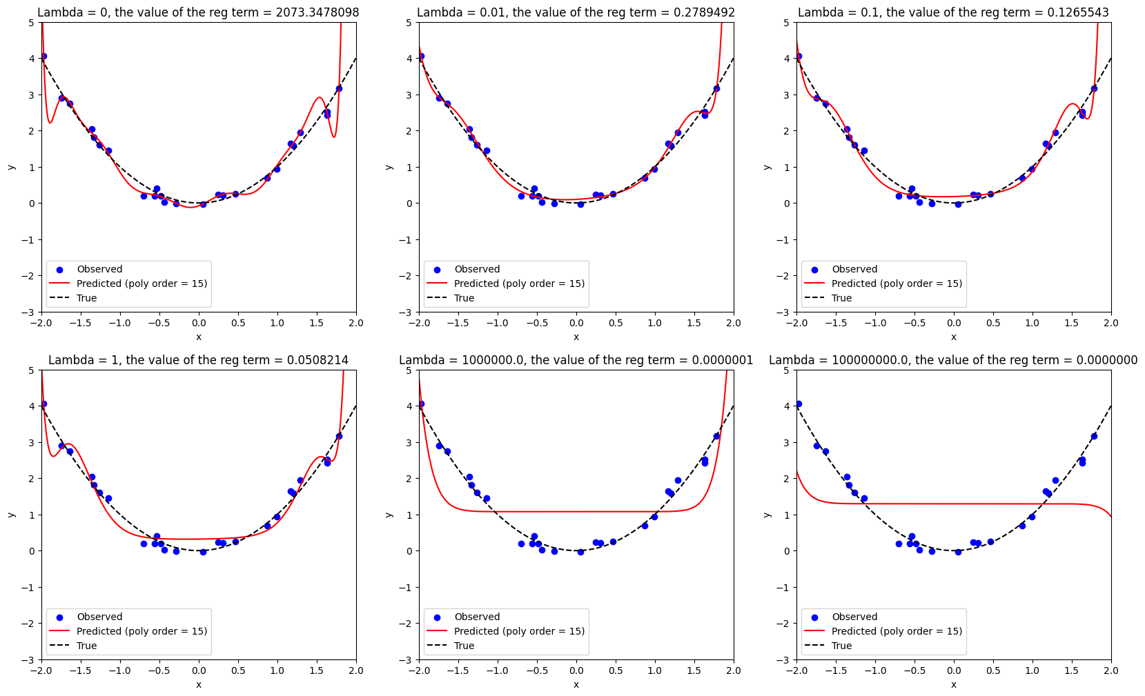
จากการทดสอบด้านบน สังเกตได้ว่า
ถ้ากำหนดให้ \(λ=0\) จะทำให้เกิดปัญหา overfitting โดยสิ่งที่โมเดลทำนาย จะ fit กับ training data (จุดสีน้ำเงิน) ได้ค่อนข้างดี ในขณะที่โมเดลไม่สามารถทำนายในบริเวณที่อยู่นอก training data ได้อย่างแม่นยำ สังเกตได้จากเส้นสีแดงมีค่าที่เปลี่ยนไปอย่างรวดเร็ว (แกว่งไปมา) และมีหน้าตาที่แตกต่างจากความสัมพันธ์ที่แท้จริง (เส้นประสีดำ) เป็นอย่างมาก
การกำหนดให้ค่า \(λ > 0\) ส่งผลให้เส้นสีแดงเริ่มแกว่งตัวน้อยลง
การเพิ่มค่า \(λ\) ให้สูงขึ้นไปเรื่อยๆ จะส่งผลให้โมเดลให้ความสนใจในการลดค่าของ regularization term มากยิ่งขึ้นเรื่อยๆ แสดงให้เห็นจากค่า \(\hat{w_0}^2 + \hat{w_1}^2 + ... + \hat{w_{15}}^2\) ที่ลดลงเรื่อยๆ
การที่โมเดลให้ความสนใจในการลดค่าของ regularization term ไปเรื่อยๆ (จากการเพิ่มค่า \(λ\)) จะส่งผลให้โมเดลสนใจที่จะ fit กับ training data (จุดสีน้ำเงิน) น้อยลงเรื่อยๆ ทำให้ได้ผลลัพธ์เป็นโมเดลที่มีหน้าตาแตกต่างจากทั้งข้อมูลที่เก็บมา (สีน้ำเงิน) และความสัมพันธ์ที่แท้จริง (เส้นประสีดำ)
จากตัวอย่างนี้ จะเห็นได้ว่า การใช้ regularization โดยที่ปรับค่า \(λ\) ได้อย่างเหมาะสม สามารถช่วยบรรเทาปัญหา overfitting ได้ในระดับหนึ่ง ซึ่งในปัจจุบัน ได้มีการคิดค้น regularization term ต่างๆ ขึ้นมามากมาย โดยที่แต่ละตัวที่คิดค้นมา ก็มีความเหมาะสมกับโจทย์ที่แตกต่างกัน ในสถานการณ์ที่แตกต่างกัน
ผู้จัดเตรียม code ใน tutorial: ดร. อิทธิ ฉัตรนันทเวช