k-Nearest Neighbors (k-NN)#
ใน tutorial ก่อนหน้านี้ เราได้เรียนรู้การทำงานของ linear regression, logistic regression, support vector machine, decision tree และ random forest ซึ่งเป็น supervised machine learning algorithms ชนิดมีโมเดลพารามิเตอร์ที่ต้องปรับเพื่อ optimize โมเดล ใน tutorial นี้ เราจะมาแนะนำ k-Nearest Neighbors (k-NN) ซึ่งเป็นตัวอย่างของ supervised machine learning algorithm ชนิด non-parametric กล่าวคือ k-NN algorithm เป็นโมเดลที่ไม่มีโมเดลพารามิเตอร์ ทำได้ทั้งการจำแนกหมวดหมู่ (classification) และ การทำนายค่า (regression) โดยอ้างอิงจากความใกล้ชิดของจุดข้อมูล (proximity) บน feature space ภายใต้สมมติฐานที่ว่า จะพบจุดข้อมูลที่คล้ายกันอยู่ใกล้กัน โดยใน tutorial นี้ เราจะแสดงการทำงานของโมเดลกับโจทย์การจำแนกหมวดหมู่
สมมติ ว่า เรามีจุดข้อมูลที่ต้องการทราบว่าอยู่ในคลาสไหน กระบวนการทำงานของ k-NN algorithm เริ่มต้นด้วยการค้นหาจุดข้อมูลเพื่อนบ้านจำนวน \(k\) จุดที่อยู่ใกล้กับจุดข้อมูลที่สนใจมากที่สุด โดยพิจารณาจากระยะห่างระหว่างจุดข้อมูลที่สนใจและจุดข้อมูลเพื่อนบ้าน จากนั้นโมเดลจะทำนายคลาสของจุดที่สนใจจากผลโหวตของจุดข้อมูลเพื่อนบ้านที่ถูกคัดเลือกมาจำนวน k จุดนั้น

k-NN algorithm adapted from ที่มา
จากรูปตัวอย่างนี้ โมเดล k-NN กำหนดจำนวนจุดข้อมูลเพื่อนบ้าน \(k=3\) ที่จะถูกใช้ในการโหวตเพื่อทำนายคลาสของจุดข้อมูลสีเหลือง โดยพบว่า ในวงเพื่อนบ้านทั้งสาม ประกอบด้วย class A จำนวน 1 จุดข้อมูล และ class B จำนวน 2 จุดข้อมูล ดังนั้น จุดข้อมูลสีเหลืองจะถูกทำนาย ว่า อยู่ใน class B
ทั้งนี้ ในตัวอย่างนี้เป็นการคำนวณระยะห่างของจุดข้อมูลด้วย Euclidean distance แต่ยังมีการพิจารณาระยะห่างแบบอื่นๆ อีก ดังต่อไปนี้

ที่มา A brief introduction to Distance Measures
สมมติว่า จุดข้อมูล 2 จุดบน feature space สามารถแทนด้วยเวกเตอร์ \(\vec{r_1}=(r_{1,1}, r_{1,2},..., r_{1,i},..., r_{1,m})\) และ \(\vec{r_2}=(r_{2,1}, r_{2,2},..., r_{2,i},..., r_{2,m})\) เมื่อ \(m\) คือ จำนวน features การหาระยะห่างระหว่างจุดข้อมูลทั้งสองสามารถคำนวณได้หลายวิธี โดยเราจะยกตัวอย่าง 3 สมการหลักที่ใช้กันทั่วไป ได้แก่
Euclidean Distance
Euclidean distance คือระยะทางเป็นเส้นตรงระหว่างจุดสองจุดใน Euclidean space จึงสามารถคำนวณได้โดยใช้ทฤษฎีพีทาโกรัส (Pythagorean theorem)
Manhattan Distance:
Manhattan distance หรือที่รู้จักกันในอีกชื่อ taxicab distance เนื่องจากพัฒนามาจากแนวคิดที่ว่า ระยะห่างระหว่างจุดสองจุดสามารถหาได้จากเส้นตาราง (grid) แทนที่จะเป็นเส้นตรง เหมือนเวลาที่รถแท็กซี่ขับไปบนถนนจากจุดหนึ่งไปสู่อีกจุดหนึ่งบนเกาะ Manhattan ที่มีการวางผังถนนเป็นเส้นตรงตัดกัน ดังนั้น Manhattan distance คำนวณระยะห่างโดยรวมความแตกต่างสัมบูรณ์ของพิกัดระหว่างจุดสองจุด
Minkowski Distance
Minkowski distance เป็นการ generalization ของ Euclidean distance และ Manhattan distance
พารามิเตอร์ \(p\ge1\) ใช้กำหนดรูปแบบของระยะทาง โดย
เมื่อ \(p=1\) Minkowski distance จะมีค่าเท่ากับ Manhattan distance
เมื่อ \(p=2\) Minkowski distance จะมีค่าเท่ากับ Euclidean distance
เมื่อ \(1<p<2\) Minkowski distance จะมีคุณลักษณะผสมผสานระหว่าง Euclidean distance และ Manhattan distance ซึ่งสามารถควบคุมได้โดยการปรับค่า \(p\)
สำหรับ classification problem เราสามารถเทรนโมเดล k-NN Classifier โดยการเรียกใช้ KNeighborsClassifier จากไลบราลี่ scikit-learn ที่มี Minkowski distance และ \(p=2\) เป็น default metric (ซึ่งก็คือ Euclidean distance)
นอกจากนี้ ยังมีการวัดระยะห่างระหว่างจุดข้อมูลด้วยวิธีอื่นๆ อีก ซึ่งสามารถกลับไปย้อนดูตัวอย่างได้จากบทเรียน Nonlinear Methods
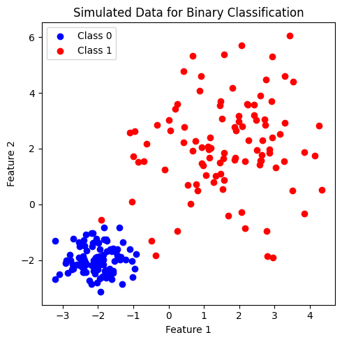
เพื่อศึกษาการทำงานของ k-NN เราจะลองสร้างชุดข้อมูลที่ประกอบไปด้วยข้อมูลจำนวน \(200\) จุด ที่ประกอบด้วย 2 features และ 2 classes ได้แก่ class 0 และ class 1 (2-class dataset for binary classification) โดยข้อมูลในแต่ละคลาสมีจำนวนเท่ากันที่ 100 จุด
import numpy as np
import matplotlib.pyplot as plt
from matplotlib import colors
from sklearn.neighbors import KNeighborsClassifier as KNC
from sklearn.inspection import DecisionBoundaryDisplay
from sklearn.model_selection import train_test_split
from sklearn.model_selection import StratifiedKFold, KFold
from sklearn.model_selection import GridSearchCV
from sklearn.preprocessing import StandardScaler
from sklearn.metrics import accuracy_score, classification_report, confusion_matrix, ConfusionMatrixDisplay

# ตั้งค่า random seed สำหรับการทำซ้ำ (reproducibility)
RANDOM_SEED = 2566
def generate_multi_class_dataset(n_classes, mean_class, std_class, n_samples):
    # สร้างชุดข้อมูลแบบ multi-class
    # ตั้งค่า random seed เพื่อให้สามารถสร้างชุดข้อมูลเดิมทุกครั้ง เพื่อใช้สำหรับการสอน
    np.random.seed(RANDOM_SEED)

    # กำหนด จำนวน features
    n_features = 2

    #  สร้างข้อมูล x สำหรับแต่ละคลาส
    x_data = []
    for label in range(n_classes):
        _ = np.random.normal(mean_class[label], std_class[label], (n_samples, n_features))
        x_data.append(_)

    # สร้างข้อมูล y หรือ labels สำหรับแต่ละคลาส
    y_data = []
    y_data.append(np.zeros(n_samples))
    for label in range(1, n_classes):
        y_data.append(label*np.ones(n_samples))

    # รวมข้อมูล x และ y จากทุกคลาส
    x = np.vstack((x_data))
    y = np.hstack(y_data)

    return x, y

# ทดลองสร้างข้อมูลโดยการเรียกใช้ generate_multi_class_dataset
# กำหนด จำนวนคลาส
n_classes = 2

# กำหนดช่วงค่า Mean และ standard deviation สำหรับแต่ละคลาส
mean_class = [[-2,-2], [2,2]]
std_class  = [[0.5,0.5], [1.5,1.5]]

# กำหนดจำนวนข้อมูล สำหรับแต่ละคลาส
n_samples = 100

# ทำการสร้างชุดข้อมูล
x, y = generate_multi_class_dataset(n_classes, mean_class, std_class,n_samples)

# Plot ข้อมูล x, y ที่มีอยู่
plt.figure(figsize = (5,5))
plt.scatter(x[y==0, 0], x[y==0, 1], c='b', label='Class 0')
plt.scatter(x[y==1, 0], x[y==1, 1], c='r', label='Class 1')
plt.xlabel('Feature 1')
plt.ylabel('Feature 2')
plt.title('Simulated Data for Binary Classification')
plt.legend()
plt.tight_layout()
plt.show()
k-NN เมื่อปรับชนิด 'metric' ที่ใช้คำนวณ distance ระหว่างจุดข้อมูล#
เราจะลองใช้ metric ที่แตกต่างกัน เพื่อดูผลของการจำแนกคลาสจาก decision boundary
# สร้างชุดโมเดล
weight = 'uniform'
models = (KNC(weights=weight, metric='euclidean'),
          KNC(weights=weight, metric='manhattan'),
          KNC(weights=weight,  metric='minkowski', p=3),
          )

# สอนโมเดลจากข้อมูล x, y ที่สร้างขึ้นก่อนหน้านี้
models = (clf.fit(x, y) for clf in models)

# ตั้งชื่อ plot ที่สอดคล้องกับชุดข้อมูล
titles = ['KNC: Euclidean distance',
          'KNC: Manhattan distance',
          'KNC: Minkowski distance (degree 3)'
          ]

# สร้าง cmap สำหรับแสดงผลตามสีแต่ละ class
cmap_2classes = colors.ListedColormap(['b', 'r'])

# plot the decision boundaries
fig, axes = plt.subplots(1,3, figsize=(4*3, 4))
for clf, title, ax in zip(models, titles, axes.flatten()):
    disp = DecisionBoundaryDisplay.from_estimator(clf,
                                                  x,
                                                  response_method="predict",
                                                  cmap=cmap_2classes,
                                                  alpha=0.5,
                                                  ax=ax,
                                                  xlabel='Feature 1',
                                                  ylabel='Feature 2',
                                                  )
    ax.scatter(x[:, 0], x[:, 1], c=y, cmap=cmap_2classes, s=20, edgecolors='k')
    ax.set_xticks(())
    ax.set_yticks(())
    ax.set_title(title)
plt.tight_layout()
plt.show()
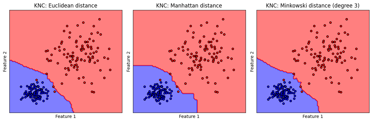
รูปแสดง decision boundary ของโมเดล k-NN เมื่อเลือกกำหนด 'metric' ที่คำนวณ distance ระหว่างจุดข้อมูลที่ต่างกันไป
จะสังเกตเห็นว่า เนื่องจากชุดข้อมูลมีการกระจายตัวแบ่งกลุ่มอย่างชัดเจน ทำให้โมเดลสามารถจำแนกข้อมูลได้คล้ายคลึงกัน ถึงแม้ว่า decision boundary มีความแตกต่างกัน
k-NN เมื่อปรับค่า n_neighbors#
จำนวนจุดข้อมูลเพื่อนบ้าน k จะกำหนดด้วย hyperparameter ชื่อ n_neighbors โดยมีค่า default เป็น n_neighbors = 5
# สร้างชุดโมเดล
models = [KNC(n_neighbors=3),
          KNC(n_neighbors=5),
          KNC(n_neighbors=25)
          ]

# สอนโมเดลจากข้อมูล x, y ที่สร้างขึ้นก่อนหน้านี้
models = [clf.fit(x, y) for clf in models]

# ตั้งชื่อ plot ที่สอดคล้องกับชุดข้อมูล
titles = ['KNC: n_neighbors=3',
          'KNC: n_neighbors=5',
          'KNC: n_neighbors=25'
          ]

# plot the decision boundaries
fig, axes = plt.subplots(1,3, figsize=(4*3, 4))
for clf, title, ax in zip(models, titles, axes.flatten()):
    disp = DecisionBoundaryDisplay.from_estimator(clf,
                                                  x,
                                                  response_method="predict",
                                                  cmap=cmap_2classes,
                                                  alpha=0.5,
                                                  ax=ax,
                                                  xlabel='Feature 1',
                                                  ylabel='Feature 2',
                                                  )
    ax.scatter(x[:, 0], x[:, 1], c=y, cmap=cmap_2classes, s=20, edgecolors='k')
    ax.set_xticks(())
    ax.set_yticks(())
    ax.set_title(title)
plt.tight_layout()
plt.show()
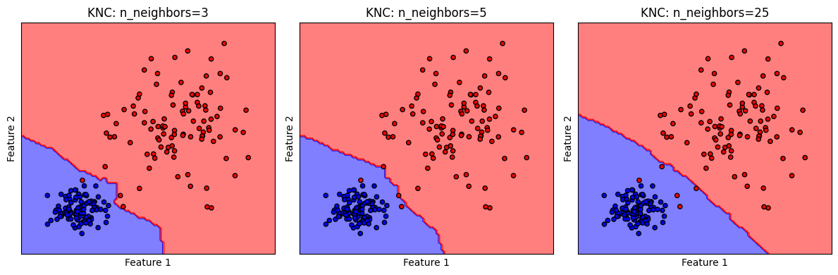
การเลือกค่า n_neighbors ที่เหมาะสมจะมีความจำเพาะต่อชุดข้อมูล ยิ่งกำหนดให้ n_neighbors มีค่ามากจะช่วยลดผลของ noise ทำให้ได้ decision boundary ที่ smooth แต่ในขณะเดียวกันก็จะทำให้ความสามารถในการจำแนกลดลง ดังจะเห็นได้จากจำนวนข้อมูล class 1 (จุดสีแดง) ที่โมเดลทำนายผิด ว่าเป็น class 0 ที่ปรากฏในพื้นที่สีฟ้า
Quiz: ถ้ากำหนดให้ n_neighbors มีค่าสูงมาก ๆ จะเป็นยังไงบ้าง
k-NN เมื่อปรับค่า weights ของจุดข้อมูล#
ที่ผ่านมา โมเดลจะจำแนกคลาสของจุดข้อมูลที่สนใจจากจุดข้อมูลที่อยู่ใกล้เคียงเป็นจำนวน n_neighbors จุด โดยเลือกคลาสที่มีจำนวนมากที่สุดเป็นคลาสของจุดข้อมูลที่สนใจ ซึ่งเป็นการให้น้ำหนักในการโหวตกับทุกจุดข้อมูลเพื่อนบ้านเท่าเทียมกัน หรือ weights='uniform' ซึ่งเป็นค่า default ของโมเดล k-NN ในไลบรารี่ scikit-learn
แต่หากเรามีสมมติฐานที่ว่า เพื่อนบ้านที่อยู่ใกล้เราที่สุดจะรู้จักเราดีที่สุด เราสามารถเลือกใช้ weights='distance' เพื่อให้โมเดลให้น้ำหนักจุดข้อมูลแต่ละจุดไม่เท่ากัน โดยอ้างอิงตามระยะห่างของจุดข้อมูลนั้นและจุดที่สนใจ
# สร้างชุดโมเดล
models = [KNC(n_neighbors=5, weights='uniform'),
          KNC(n_neighbors=5, weights='distance')
          ]

# สอนโมเดลจากข้อมูล x, y ที่สร้างขึ้นก่อนหน้านี้
models = [clf.fit(x, y) for clf in models]

# ตั้งชื่อ plot ที่สอดคล้องกับชุดข้อมูล
titles = ['KNN with n_neighbors=5, weights="uniform"',
          'KNN with n_neighbors=5, weights="distance"'
          ]

# plot the decision boundaries
fig, axes = plt.subplots(1,2, figsize=(8, 4))
for clf, title, ax in zip(models, titles, axes.flatten()):
    disp = DecisionBoundaryDisplay.from_estimator(clf,
                                                  x,
                                                  response_method="predict",
                                                  cmap=cmap_2classes,
                                                  alpha=0.5,
                                                  ax=ax,
                                                  xlabel='Feature 1',
                                                  ylabel='Feature 2',
                                                  )
    ax.scatter(x[:, 0], x[:, 1], c=y, cmap=cmap_2classes, s=20, edgecolors='k')
    ax.set_xticks(())
    ax.set_yticks(())
    ax.set_title(title)
plt.tight_layout()
plt.show()
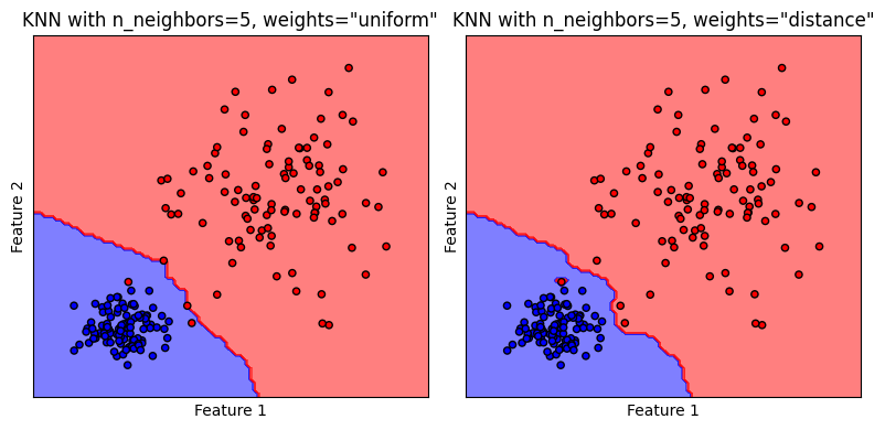
รูปแสดง decision boundary ของโมเดล k-NN เมื่อเลือกกำหนด weights ต่างกัน
Quiz: จากรูปที่มีการเปรียบเทียบ decision boundary สามารถอธิบายได้หรือไม่ว่า weights ที่ต่างกันมีผลอย่างไร
k-NN Classification Pipeline#
ต่อไปเราจะลองพัฒนาโมเดล k-NN อย่างครบกระบวนการ ด้วยชุดข้อมูลที่จะสร้างขึ้น
Generate 3-class Dataset#
# สร้างข้อมูลโดยการเรียกใช้ generate_multi_class_dataset
# กำหนด จำนวนคลาส
n_classes = 3

# กำหนดช่วงค่า Mean และ standard deviation สำหรับแต่ละคลาส
mean_class = [[-2,2], [1,0], [2,1]]
std_class  = [[0.5,0.5], [0.75,0.75],[0.75,0.5]]

# กำหนดจำนวนข้อมูล สำหรับแต่ละคลาส
n_samples = 200

# ทำการสร้างชุดข้อมูล
x, y = generate_multi_class_dataset(n_classes, mean_class, std_class,n_samples)

# Plot ข้อมูล x, y ที่สร้างขึ้น
plt.figure(figsize = (5,5))
color_list = ['b','r','g']
cmap_3classes = colors.ListedColormap(color_list)
for label in range(n_classes):
    plt.scatter(x[y==label, 0], x[y==label, 1], c=color_list[label], label='Class '+str(label))

plt.xlabel('Feature 1')
plt.ylabel('Feature 2')
plt.title('Simulated 3-class dataset')
plt.legend()
plt.tight_layout()
plt.show()
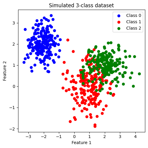
ข้อมูลที่สร้างขึ้นมีประกอบด้วย 2 features และ 3 classes (class: 0, 1, 2) โดยข้อมูลในแต่ละคลาสมีจำนวนเท่ากันที่ 200 จุด เราจะพัฒนาโมเดล k-NN เพื่อจำแนกข้อมูลแต่ละคลาสออกจากกัน
เมื่อสังเกตการกระจายตัวของข้อมูล พบว่า class 0 มีการกระจายข้อมูลแบ่งแยกออกมาอย่างเห็นได้ชัด ในขณะที่ class 1 และ class 2 จะกระจายตัวอยู่ร่วมกัน
แบ่งข้อมูลเป็น training data และ test data#
โดยใช้ train_test_split จากไลบรารี่ scikit-learn
ในตัวอย่างนี้เราจะใช้ default value ซึ่งจะ shuffle ข้อมูลก่อนแบ่งข้อมูล และ ไม่ stratify (ไม่กำกับสัดส่วนของคลาสใน training data และ test data)
อย่างไรก็ดี ในกรณีที่ข้อมูลประกอบด้วยคลาสต่างๆ ที่มีสัดส่วนต่างกันอย่างมาก (imbalanced dataset) การทำ stratify มีความจำเป็นอย่างมากเพื่อคงสัดส่วนของแต่ละคลาส ใน training data และ test data
# สร้าง training data และ test data โดยแบ่งจากชุดข้อมูล x,y
x_train, x_test, y_train, y_test = train_test_split(x, y, test_size=0.2,
                                                    stratify=None,
                                                    shuffle=True,
                                                    random_state=RANDOM_SEED)

print('Train set: จำนวนข้อมูล แบ่งกลุ่มตาม class label')
unique, counts = np.unique(y_train, return_counts=True)
print(np.asarray((unique, counts)).T)

print('Test set: จำนวนข้อมูล แบ่งกลุ่มตาม class label')
unique, counts = np.unique(y_test, return_counts=True)
print(np.asarray((unique, counts)).T)
Train set: จำนวนข้อมูล แบ่งกลุ่มตาม class label
[[  0. 169.]
 [  1. 155.]
 [  2. 156.]]
Test set: จำนวนข้อมูล แบ่งกลุ่มตาม class label
[[ 0. 31.]
 [ 1. 45.]
 [ 2. 44.]]
ทำการ standardize ข้อมูลทั้งหมด#
ใช้ mean และ standard deviation (SD) จาก training data ในการ standardize test set เพื่อป้องกัน information leak
# สร้าง standardized scaler จาก features ใน training data
x_scaler = StandardScaler().fit(x_train)

# scale ค่า features ใน training data และ test data
x_train = x_scaler.transform(x_train)
x_test  = x_scaler.transform(x_test)
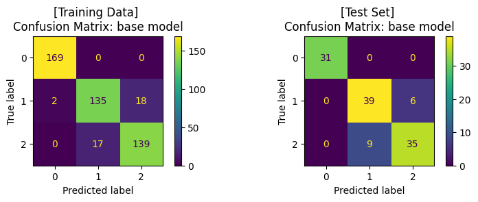
เทรนโมเดล ด้วย base model (default hyperparameter)#
fig, (ax1, ax2) = plt.subplots(1, 2, figsize=(8, 3))

# สร้างโมเดล
base_clf = KNC()

# สอนโมเดลด้วย training data
base_clf.fit(x_train,y_train)

# ให้โมเดลทำนาย training data
y_pred = base_clf.predict(x_train)

# แสดงผล classification ของโมเดลจาก training data
print('Training Set: Classification report')
print(classification_report(y_train, y_pred))

# คำนวนและแสดงผล confusion matrix ของ training data
cm = confusion_matrix(y_train, y_pred)
display = ConfusionMatrixDisplay(confusion_matrix=cm)
display.plot(ax=ax1)
ax1.set_title('[Training Data] \nConfusion Matrix: base model')

# ให้โมเดลทำนาย test data
y_pred = base_clf.predict(x_test)

# แสดงผล classification ของโมเดล
print('\nTest Set: Classification report')
print(classification_report(y_test, y_pred))

# คำนวนและแสดงผล confusion matrix ของ test set
cm = confusion_matrix(y_test, y_pred)
display = ConfusionMatrixDisplay(confusion_matrix=cm)
display.plot(ax=ax2)
ax2.set_title('[Test Set] \nConfusion Matrix: base model')

plt.tight_layout()
plt.show()
Training Set: Classification report
              precision    recall  f1-score   support

         0.0       0.99      1.00      0.99       169
         1.0       0.89      0.87      0.88       155
         2.0       0.89      0.89      0.89       156

    accuracy                           0.92       480
   macro avg       0.92      0.92      0.92       480
weighted avg       0.92      0.92      0.92       480


Test Set: Classification report
              precision    recall  f1-score   support

         0.0       1.00      1.00      1.00        31
         1.0       0.81      0.87      0.84        45
         2.0       0.85      0.80      0.82        44

    accuracy                           0.88       120
   macro avg       0.89      0.89      0.89       120
weighted avg       0.88      0.88      0.87       120
ปรับแต่งโมเดล (Hyperparameter Tuning) ด้วย GridSearchCV และ train โมเดล#
โดยเราจะปรับแต่งโมเดล โดย tune 2 hyperparameters ที่สำคัญของโมเดล k-NN ได้แก่
weightsn_neighbors
ในไลบรารี่ scikit-learn ยังมีวิธีการอื่นๆ ในการปรับแต่งโมเดล เช่น
fig, (ax1, ax2) = plt.subplots(1, 2, figsize=(8, 3))

# กำหนดช่วงค่า hyperparameters ในรูปแบบ dictionary
clf_params = {'weights': ['uniform','distance'],
              'n_neighbors': [3, 5, 7, 9, 11]
              }

# แบ่งข้อมูล training data ด้วย 5-fold cross-validation เพื่อ tune hyperparameter
cv_splitter = KFold(n_splits=5, shuffle=True, random_state=RANDOM_SEED)

# ใช้ GridSearchCV เพื่อสอนโมเดลจากชุดค่า hyperparameters จาก clf_params
# และคำนวณค่า accuracy ของแต่ละโมเดล เพื่อเลือกชุด hyperparameters ที่ดีที่สุด
# โดยใช้เทคนิค cross-validation ในการแบ่งกลุ่ม validation data จาก training data
tuned_clf = GridSearchCV(estimator=base_clf, param_grid=clf_params,
                             scoring=['accuracy'], refit='accuracy', cv=cv_splitter)

# fit โมเดลด้วย training data และ ให้โมเดลทำนายค่า y จาก training data
tuned_clf.fit(x_train, y_train)
y_pred = tuned_clf.predict(x_train)

# แสดงผล hyperparameters ที่ดีที่สุด และ cross-validation score
print('Best hyperparameters: {}'.format(tuned_clf.best_params_))
print("Best cross-validation score: {:.2f}".format(tuned_clf.best_score_))

# แสดงผล classification ของโมเดลจาก training data
print('Training Set: Classification report')
print(classification_report(y_train, y_pred))

# คำนวนและแสดงผล confusion matrix ของโมเดลจาก training data
cm = confusion_matrix(y_train, y_pred)
display = ConfusionMatrixDisplay(confusion_matrix=cm)
display.plot(ax=ax1)
ax1.set_title('[Training Data] \nConfusion Matrix: tuned model')

# ให้โมเดลทำนายค่า y จาก test data
y_pred = tuned_clf.predict(x_test)

# แสดงผล classification ของโมเดล จาก test data
print('\nTest Set: Classification report')
print(classification_report(y_test, y_pred))
# คำนวนและแสดงผล confusion matrix จาก test data
cm = confusion_matrix(y_test, y_pred)
display = ConfusionMatrixDisplay(confusion_matrix=cm)
display.plot(ax=ax2)
ax2.set_title('[Test Set] \nConfusion Matrix: tuned model')

plt.show()
Best hyperparameters: {'n_neighbors': 7, 'weights': 'distance'}
Best cross-validation score: 0.90
Training Set: Classification report
              precision    recall  f1-score   support

         0.0       1.00      1.00      1.00       169
         1.0       1.00      1.00      1.00       155
         2.0       1.00      1.00      1.00       156

    accuracy                           1.00       480
   macro avg       1.00      1.00      1.00       480
weighted avg       1.00      1.00      1.00       480


Test Set: Classification report
              precision    recall  f1-score   support

         0.0       1.00      1.00      1.00        31
         1.0       0.83      0.89      0.86        45
         2.0       0.88      0.82      0.85        44

    accuracy                           0.89       120
   macro avg       0.90      0.90      0.90       120
weighted avg       0.89      0.89      0.89       120
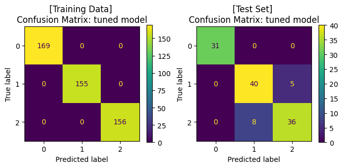
จะสังเกตได้ว่า เมื่อมีการปรับจูน hyperparameters ของโมเดลให้มีความเหมาะสมแล้ว เราได้โมเดลที่เรียนรู้จากข้อมูลชุดเดิม แล้วสามารถทำนาย test data ได้ค่า accuracy ที่สูงขึ้น โดยเมื่อพิจารณา Confusion Matrix จะพบว่า โมเดลสามารถจำแนกข้อมูล class 1 และ class 2 ได้ดีขึ้น
Decision Boundary#
เราจะมาลองดู decision boundary ของโมเดลบน training data และ test data
# plot the decision boundaries
fig, axes = plt.subplots(1,2, figsize=(7, 4))
titles = ['[Training Data] \nk-NN: Decision boundary', '[Test Data] \nk-NN: Decision boundary']
for x, y, title, ax in zip([x_train, x_test], [y_train, y_test], titles, axes.flatten()):
    disp = DecisionBoundaryDisplay.from_estimator(tuned_clf,
                                                  x,
                                                  response_method="predict",
                                                  cmap=cmap_3classes,
                                                  alpha=0.5,
                                                  ax=ax,
                                                  xlabel='Feature 1',
                                                  ylabel='Feature 2',
                                                  )
    ax.scatter(x[:, 0], x[:, 1], c=y, cmap=cmap_3classes, s=20, edgecolors='k')
    ax.set_xticks(())
    ax.set_yticks(())
    ax.set_title(title)
plt.tight_layout()
plt.show()
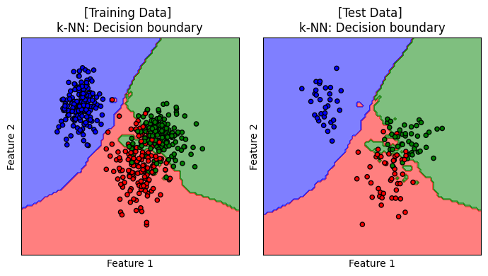
แสดง decision boundary ของโมเดล k-NN เมื่อ n_neighbors=7 และ weights='distance' ซึ่งเป็นโมเดลที่ได้รับการปรับจูนให้เหมาะสมกับการเรียนรู้จากชุดข้อมูลนี้
Discuss: ข้อเสียของโมเดล k-NN
เทคนิคนี้ต้องจัดเก็บ training set ทั้งอัน รวมถึงต้องคำนวณ distance ระหว่างแต่ละคู่จุดข้อมูล ซึ่งจะเป็นปัญหาอย่างมากเมื่อเรามีจำนวนจุดข้อมูลใน training set จำนวนมาก
ในทางปฏิบัติ เวลาที่จะหา neighbors ใกล้ตัวของจุดข้อมูล เราสามารถใช้เทคนิค tree-based search structures เพื่อให้สามารถหา neighbors เหล่านั้นได้อย่างรวดเร็วกว่าการไปไล่ดูทุกจุดข้อมูลใน training set แต่ก็ต้องแลกมากับความคาดเคลื่อนที่อาจเกิดขึ้นได้
ผู้จัดเตรียม code ใน tutorial: ดร. กนกกร พิมพ์เจริญ